CASSA Workshop 1: Unclouding the thousand eyes of an Array Radio Telescope

The Center for Astronomy, Space Science and Astrophysics (CASSA) aims to build an academic institution for astronomy in Bangladesh that is truly part of the international astronomy community. The goal is for astronomy here to operate just as it does in other countries. Our connection to the global community comes through CASSA’s associate members—many of whom are faculty or postdocs based in North America. We want to connect university students in Bangladesh with them in meaningful and productive ways. CASSA will be a confluence, where old rivers from abroad merge with new rivers at home, creating a new future shaped by the influence of the past.

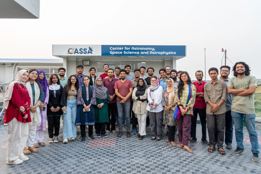
To bring together students from various universities across the country and introduce them to modern astronomical methods, CASSA will host regular workshops and mini-courses. Our first such effort, acting as a pathfinder, was held on May 2–3, 2025, at the rooftop CASSA office in the main academic building of Independent University, Bangladesh (IUB). A total of 30 students from 15 universities in Bangladesh attended the two-day workshop, where they participated in lectures and hands-on work.

The theme of the workshop was Array Radio Telescopes (ART)—radio telescopes built from a collection of antennas working together. The choice of topic was shaped by the fact that I am currently CASSA’s only in-house astronomer, and my primary research field is ART. I don’t call myself a radio astronomer, since I also work on X-ray astronomy, and without connecting different wavelengths, one cannot experience the full joy of this science. However, I kept the workshop focused on ART because we’ve recently been building a small array next to the CASSA office, which has kept us deeply engaged with radio astronomy. Given this context, I felt radio astronomy was the topic I could most enthusiastically and effectively share with students, even with minimal preparation.

On the first day of the workshop, I gave three lectures: one on radio astronomy, one on ART, and one on radio antenna beams. Students were divided into eight groups of four to five members. In the afternoon, each group began setting up their project on CASSA’s high-performance computing (HPC) server, named Timaeus. Early on the second day, I gave a lecture on modeling the beam of a LOFAR (Low Frequency Array) station in the Netherlands using Zernike polynomials. The rest of the day was spent with the eight groups working on that model. At the end of the day, each group presented their results to everyone.

The purpose of this write-up is to share the experience of those two days from the perspective of an instructor. I will also summarize the lecture topics here.

1. Day One

Around 100 students applied for CASSA Workshop 1. Based on relevant coursework, CGPA, and other criteria in their applications, we selected 45 students. I had some doubts about whether everyone would actually show up, but I figured that if even 30 out of 45 came, the workshop would be a success. I had three students who earned an ‘A’ in my Summer 2024 Radio Astronomy course at IUB—so I brought them in as Teaching Assistants (TAs) for the workshop.

On May 2nd, I arrived at the CASSA office at 9:05 AM—true to my usual sick habit of always being five minutes late. I always try to be 10 minutes early and end up being 10 minutes late. When I got there, I saw that quite a few students were already waiting outside; the door was locked and they couldn’t get in.

The first hour, from 9:00 to 10:00, was set aside for icebreaking. Students would arrive, have tea, and get to know each other. I wasn’t disappointed—by 9:30, most of them had already arrived. I kept track of everyone’s arrival time in a Google Sheet. After 30 students had arrived, I initially formed six groups of five students each. But then about 10 more arrived, and I had to expand it to eight groups in total. The groups sat at eight tables in the office.

I had originally designed the CASSA office with my course ‘Our Cosmic History‘ in mind. In that course, I have 40 students divided into eight groups of five. Throughout the trimester, each group sits at the same table because there’s a group exercise after every lecture. That classroom design turned out to be perfect for the workshop, too.

1.1 Radio Astronomy

After the icebreaker, at 10:00 AM, I gave the first one-hour lecture on the basics of radio astronomy. The topics covered included light, mechanisms of light emission and detection, and units for measuring light.

Light has to be described both as particles (photons) and as electromagnetic waves. In high-frequency X-ray astronomy, it’s more convenient to describe light as particles, whereas in low-frequency radio astronomy, it’s more useful to think of light as waves. Since our workshop focused on radio astronomy, the wave nature of light was most relevant to us.

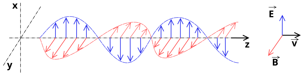
Astronomers across all frequency bands visualize the sky as an XY plane, with the direction of incoming light along the Z-axis—that is, along our line of sight. In this XY plane, oscillations in the electric field (denoted as $\mathbf{E}$ in blue) and the magnetic field ($\mathbf{B}$ in red) create a wave that propagates along the Z-axis.

I often use the analogy of a rope. If one end of a rope is tied to a pole and I shake the other end up and down, a wave will travel along the rope toward the pole. In this analogy, my hand represents the electric charge, and the wave is the light. I’m moving my hand within the XY plane, say along the Y-axis, and the resulting wave travels along the Z-axis. In the diagram, the electric field oscillates along the X-axis, while the magnetic field oscillates along the Y-axis. In practice, for light, the magnitude of the magnetic field is so much smaller than that of the electric field that telescopes primarily detect the electric component of the wave.

But that brings us to a deeper question: Why does the electric field oscillate at all? In the rope example, a wave exists only because I’m physically shaking one end. If an electric field line is like a rope, someone has to “shake” its end to generate a wave. So—who’s shaking it?

The answer is simple: electric charge. An electric field line originates from a charge and radiates out to infinity. If the charge moves at a constant speed, the field lines remain steady, and no wave is produced. But if the charge accelerates—meaning its velocity changes—then a disturbance propagates along those field lines in the form of a wave.

The charge is analogous to my hand in the rope analogy. Just like I had to accelerate my hand to generate a wave in the rope, a charge must accelerate to produce light. This acceleration of electric charges is the fundamental cause behind all light emission.

So, light can be emitted from any astronomical object due to the acceleration of a large number of electric charges within it. This light, or more precisely the electromagnetic wave, then travels through space and eventually reaches us, where we detect it using telescopes. The way a radio telescope detects such radiation is shown in the diagram above.

Any telescope typically has four main parts: the collector, the detector, the processor, and the mount. The collector reflects and focuses incoming radiation onto the focal plane. At that focal plane, the detector converts the incoming photons to electrons, or the electric field into current. The processor then takes this electron or current signal and processes it to generate a final image. The collector-detector system sits on a mount or pedestal. Often, the mount has a drive system that allows the telescope to rotate or point toward a desired direction. In the diagram above, we see only a simple representation of the detector, since that is the most important part for understanding radio telescopes in the context of the workshop.

In radio astronomy, the detector is often called a feed. To measure the complete electric field in the XY plane, we must be able to independently measure both of its components: X and Y. That is why a feed typically has two elements, one for each component. The simplest such feed is the dipole, which was first built by Heinrich Hertz. The image shows only the dipole that detects the Y component. In practice, two such dipoles are arranged perpendicular to each other in the XY plane, and together they are referred to as a cross-dipole.

The animation shows how one component of the field induces a signal in one dipole. As the field oscillates, it generates opposite currents on the two ends of the dipole. That’s why it’s called a dipole. This current arises due to a potential difference between the two ends of the antenna, which can be measured as a voltage $V$. According to Ohm’s law, the ratio of voltage to current depends on the resistance $R$ of the circuit. The voltages from the X and Y feeds together form the raw data of a radio telescope. In short: a radio telescope measures the voltage of the sky.

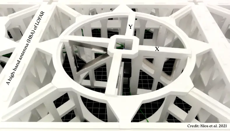
Here, a high-band antenna of LOFAR is shown. Perpendicular X and Y feeds are visible. The voltages of these two feeds are denoted as $V_{xx}$ and $V_{yy}$, respectively. The X feed is supposed to detect only the X component of the electric field, and the Y feed only the Y component, but in practice, some part of the Y component leaks into the X feed, and some part of the X component leaks into the Y feed. Because of this, two more voltage components, $V_{xy}$ and $V_{yx}$, are obtained; these are called cross-talk. These four components are stored in a 2×2 Jones matrix:

$$ \mathbf{V} = \begin{pmatrix}
V_{xx} & V_{xy} \\
V_{yx} & V_{yy}
\end{pmatrix}$$

and each value in this matrix is a complex number. The electric field value is always real, but to work with all the information of a time-varying electric field, complex numbers are required, because the phase difference between one wave and another is stored in the imaginary part. If the real part gives the magnitude of the field, then the complex part gives the wave’s phase or arrival time. If phase delay or time delay is stored using complex numbers, the calculation becomes much easier. A time-dependent electric field,

$$ E(t) = E_0 \cos(\omega t + \phi) $$

where $E_0$ is its amplitude, $\omega$ is the angular frequency (unit: radians/second), and $\phi$ is the phase. We write the same as a complex number as

$$ \tilde{E}(t) = E_0 e^{i(\omega t + \phi)} $$

where $e^{i\omega t} = \cos(\omega t) + i\sin(\omega t)$, $e$ is Euler’s number, and $i=\sqrt{-1}$ is the imaginary unit. If one wants to work with real numbers, amplitude and phase have to be stored separately, but with a complex number, all the information of amplitude and phase can be contained in a single number.

In the workshop, a student asked a good question about the reality of complex numbers. Are the electric field and the resulting voltages truly complex—do they really contain imaginary numbers—or are complex numbers used here only for computational convenience? At any given time, the values of the field and voltage are real, but their variation with time cannot be properly described without complex numbers. One might argue that amplitude and phase can just be stored separately—what’s the point of complicating things with complex numbers? But in fact, calculations become so much simpler with complex numbers that it’s hard not to think of reality itself as complex. When, instead of one antenna, we think of an array of many antennas, the importance of complex numbers becomes even more evident—this was the topic of my next lecture.

But before that, I introduced the idea of light measurement units by explaining the two most important parameters of any telescope: resolution and sensitivity. How small an object a telescope can see depends on its resolution, and how faint an object it can detect depends on its sensitivity. Sensitivity is given as a flux. For example, the sensitivity of South Africa’s telescope MeerKAT is about 5 micro-jansky (Jy), meaning any object brighter than 5 micro-Jy is detectable by it. But what is a Jy? Jy is the most fundamental unit in radio astronomy, named after Karl Jansky, one of the founders of radio astronomy and an electrical engineer.

We measure radio light in Jy units because the intensity of radio light is much lower than that of visible light. While the Sun’s power in visible light is about $10^{+26}$ W, one Jy is $10^{-26}$ W m$^{-2}$ Hz$^{-1}$, extremely small. At around 1 GHz frequency in our sky, the Sun’s flux density is approximately 1000 Jy, and the brightest radio object in the sky, Cassiopeia A (Cas A), has a flux density of about 3000 Jy.

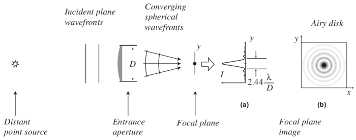
To explain resolution, I always use this diagram from Frederick Chromey’s book; it shows the process of light arriving at a telescope’s aperture (another name for antenna) from a point source like a star. All stars appear point-like in the sky, but after taking an image with any telescope, the resulting image looks like the Airy disk shown in panel (b). This wave pattern from a point source arises due to the diffraction of light at the aperture. Simply put, light bends at the two edges of the aperture—or, new spherical wavefronts are generated—and due to interference among multiple waves, the resulting image appears as an Airy disk. A one-dimensional profile of this disk is shown in panel (a). Another name for this disk is the Point Spread Function (PSF), and the angular radius of its central main lobe is called the resolution ($\alpha$).

MeerKAT’s resolution can often be as fine as 5 arcseconds (1 arcsecond is 1/3600th of a degree). This means that if an image of a star-like point source is taken with MeerKAT, the angular radius of the main lobe of the Airy disk that appears in the image will be 5 arcseconds. So, if an object in the sky has an angular size smaller than 5 arcseconds, MeerKAT won’t be able to separate it from its surrounding background—it won’t be able to resolve it. That’s why it’s called resolution. From panel (a), we see that the angular radius of the Airy disk or PSF’s main lobe is given by:

$$ \alpha = 1.22 \frac{\lambda}{D} $$

which is the resolution of a telescope with diameter $D$ at wavelength $\lambda$. As the diameter of the telescope’s collector increases, $\alpha$ decreases—meaning the resolution improves. But since the wavelength of radio waves is much longer, achieving good resolution with a radio telescope requires a very large diameter. The diameter of the largest optical telescope is 10.4 meters, and at 600 terahertz its resolution is 0.01 arcseconds. On the other hand, the largest single-dish radio telescope has a diameter of 500 meters, and at 1500 megahertz, its resolution is around 80 arcseconds. Even with a 500-meter collector in radio, it cannot match the resolution of a 10-meter optical collector.

Therefore, the only way to improve resolution in radio is to use an array of widely spaced antennas. In such cases, the resolution no longer depends on the diameter of a single antenna, but rather on the distance between the two farthest antennas in the array.

1.2. Array Radio Telescope (ART)

After a tea break, I tried to explain to everyone the concept of an array made of multiple antennas. At that time, we were deploying a small array radio telescope called the Small Transient Array Radio Telescope (START) just outside the CASSA office. Shoaib from the Fab Lab was still working outside then. This was an array of 24 antennas, but during the workshop, we worked with the LOFAR telescope in the Netherlands, which has nearly 50,000 high-band antennas. A combination of two antennas is called an interferometer, and many such interferometers together make up an array.

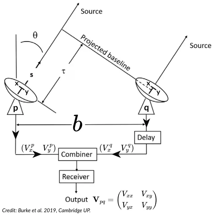
Let’s say two antennas, $p$ and $q$, are observing light coming from a source in the sky at an angle $\theta$ with respect to the vertical direction (zenith). The light reaches antenna $q$ first, and after a time delay of $\tau$, it reaches antenna $p$. To correct for this delay, we need to add a time delay to the observation at antenna $q$.

Each antenna has both X and Y feeds in the focal plane. The combiner’s job is to correlate the voltages from the X and Y feeds of both antennas and send the result to the receiver. The data finally generated in the receiver is called the visibility $V_{pq}$, which is the correlation of the observations from the two antennas separated by a distance $b$ (called the baseline). This too is a Jones matrix, but here each element is the correlation between the data from the two antennas. That is, $V_{xx}$ refers to the cross-correlation between the X-feed voltage of antenna $p$ and the X-feed voltage of antenna $q$.

In the 1930s, Dutch physicists Pieter Hendrik van Cittert and Frits Zernike discovered that, under certain conditions, the Fourier transform of the intensity distribution of light from a very distant source is equal to the complex interferometric visibility of that light. This means that the complex visibility obtained from a baseline between two antennas is a direct Fourier transform of the sky. In other words, an interferometer doesn’t capture a direct image of the sky—it samples the Fourier transform of the sky instead.

Fourier transform refers to representing any image or signal using a combination of many sine and cosine functions with different frequencies and amplitudes. A sinusoidal function of a specific frequency and amplitude is called a Fourier mode. A baseline detects one such Fourier mode of the sky. The complex visibility measured by an ART is described by the Radio Interferometric Measurement Equation (RIME):

$$ \mathbf{V}_{pq}(u,v) = \iint_{l,m} \mathbf{B}_p \ \mathbf{E}(l,m) \ e^{-2\pi i(ul+vm)} \ \mathbf{B}_q^H \ dl \ dm $$

Here, $l,m$ are the sky coordinates (cosines of the right ascension and declination directions), $u,v$ are the coordinates of a baseline on Earth’s surface, $\mathbf{B}$ is the beam of a single antenna (i.e., its sensitivity in different directions), and $^H$ denotes the Hermitian conjugate or adjoint. The brightness matrix of the object in the sky is

$$ \mathbf{E} = \begin{pmatrix} E_{xx} & E_{xy} \\
E_{yx} & E_{yy}
\end{pmatrix}$$

where $E_{xx}$ is the auto-correlation of the X component of the electric field coming from the sky. This is the 2D version of RIME, where the Fourier relationship between sky and ground is explicitly shown. But to understand the coordinates of the baseline, we need to understand the uv-plane and uv-coverage, and for that, we have to consider arrays made of many antennas instead of just a two-antenna interferometer. In the workshop, I used a software called friendly VRI to show array configurations—and I’ll use it here too. This tool can simulate mock observations of some of the world’s largest ARTs on a small scale.

I have selected India’s Giant Meterwave Radio Telescope (GMRT) for the observations. This array consists of 30 parabolic mesh antennas arranged in a Y-configuration, with each antenna having a diameter of 45 meters. The positions of the antennas are shown in the top-left corner, where the x-axis represents the relative distance in kilometers along the east-west direction, and the y-axis represents the distance along the north-south direction. I have selected an hour angle range of -4 to +5 hours, meaning a setup for approximately 11 hours of observation. For the model image, I have chosen an image of a radio galaxy with two lobes emerging from the black hole in the center. Instead of the galaxy, I could have used my own image as well. This software generates the expected appearance of any image when observed with an array. From 30 antennas, we get a total of 30 × 29 / 2 = 435 unique pairs. Each pair represents a baseline.

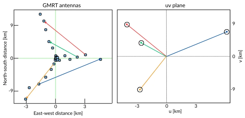
Each pair’s baseline can be thought of as a vector. Four such vectors are shown above. When these vectors are translated to a common origin, the resulting plane is called the $uv$-plane, because its x-axis represents $u$ and its y-axis represents $v$. These coordinates are used in the RIME. Knowing the tip of a vector allows us to determine its direction and length, so only the tips are shown in the right panel of the image as circles. Now, if we remove the lines of the vectors and keep only the tips, it becomes easier to understand the track of each tip. Since the Earth completes one rotation every 24 hours, each tip will describe a complete ellipse relative to an object in the sky. Given that we have an 11-hour observation, each tip will trace out approximately half of an ellipse.

In this way, the pattern formed in the uv-plane during 11 hours of observation is called the uv-coverage, which is shown in the middle panel of the top row in the image below. Clicking the “Do Observation” button in the Friendly VRI software will generate the images shown below.

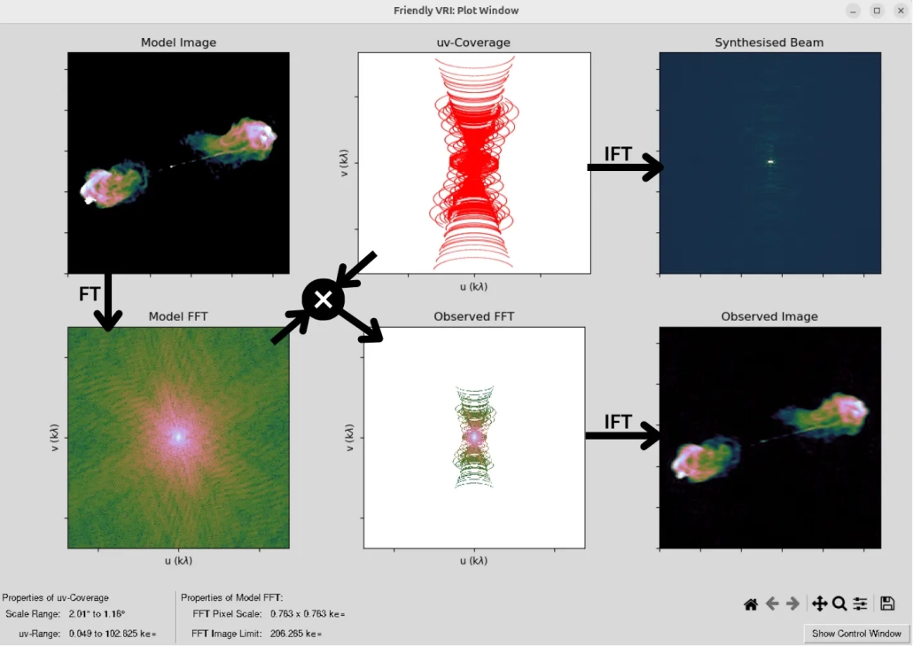
This image shows each step of the Friendly VRI simulation. The model image is the target object we want to image using the array. Its Fourier transform gives the model FFT (Fast Fourier Transform). Not all Fourier modes in the model FFT can be sampled by the array; only those falling within the $uv$-coverage will be sampled. This is effectively the result of multiplying the model FFT with the $uv$-coverage mask. Multiplying in the Fourier domain corresponds to a convolution in the image domain. The result of this convolution is our observed FFT, which, when inverse Fourier transformed (IFT), gives the observed image.

It is useful to note that the IFT of the $uv$-coverage alone yields the synthesized beam of the array. In contrast, the beam of a single antenna is called the primary beam. The field of view (FoV) of an image taken with the array is determined by the diameter of the main lobe of the primary beam, while the resolution is determined by the diameter of the main lobe of the synthesized beam. The size of the primary beam depends on the diameter $D$ of a single antenna via $\lambda/D$, and the size of the synthesized beam depends on the length $b$ of the longest baseline via $\lambda/b$.

If each GMRT antenna is 45 meters in diameter and the wavelength is 21 cm, then the field of view is approximately 16 arcminutes, meaning that the image will show a 16-arcminute-wide patch of sky; note that the Moon’s diameter is about 30 arcminutes. And if the longest baseline in the array is 25 km, then at the same wavelength, the resolution will be approximately 1.7 arcseconds.

The raw data from the array are complex visibilities, whose equation is known as the RIME. How many visibilities are obtained from the observation described above? For the 435 baselines, one visibility is sampled every 300 seconds over 11 hours, so the total number of visibilities is approximately 57,000. In the “Observed FFT” panel above, each dot’s color shows the visibility observed by the baseline at that $uv$-coordinate.

These visibilities must first be calibrated to remove all systematic effects. Then, all clean visibilities are averaged into a grid and inverse Fourier transformed to produce the final image. One major step in the calibration is to remove the effect of the antenna’s primary beam $\mathbf{B}(l,m)$ from the RIME. For that, we need to understand the primary beams of each antenna in the array, which is what we started to do after lunch.

1.3. Antenna Primary Beam

After the lunch break, from 2:30 PM, the discussion started on the antenna primary beam, and we had to focus on LOFAR. The main objective of the workshop is to model the beam of a LOFAR station. This array has thousands of antennas spread across Europe.

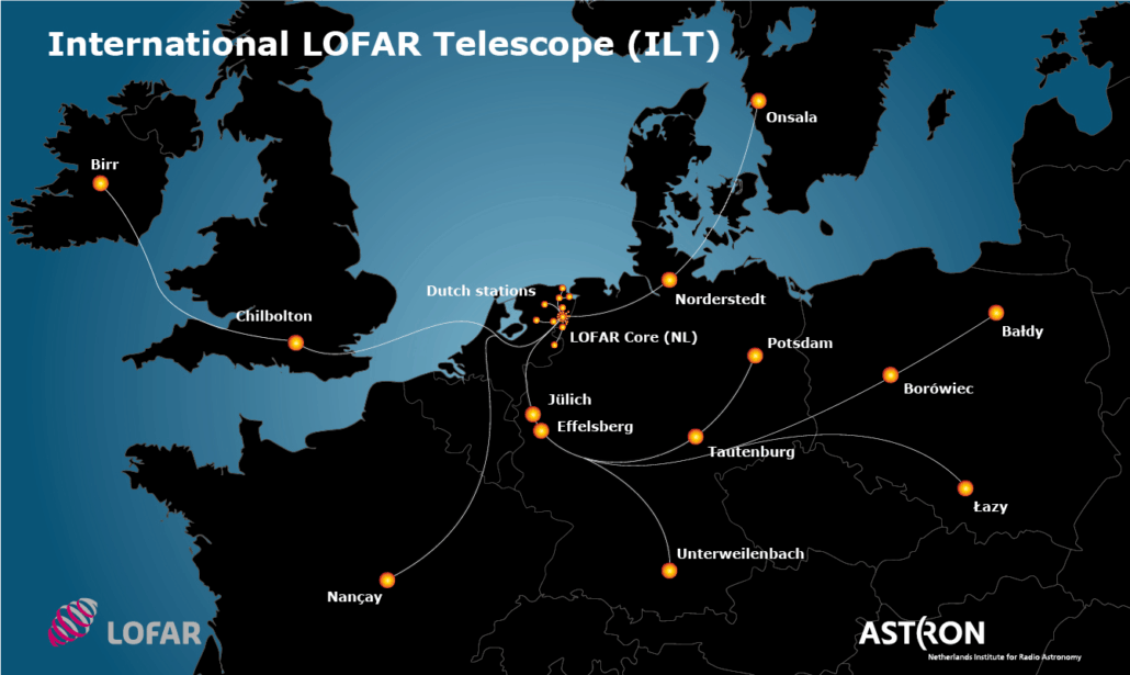
From the core in the Netherlands, four spiral arms extend up to about 500 km. There are stations from Onsala in Sweden in the north to Nançay in France and Unterweilenbach in Germany in the south, and from Birr in Ireland in the west to Baldy in Poland in the east. Because of this, LOFAR’s longest baseline is about 1000 km. The high-band antennas (HBA) observe in the range of 110 to 240 MHz. Inside the Netherlands, LOFAR has 30 core stations within 3.5 km, each containing two HBA substations. A single HBA core station consists of a total of 384 antennas arranged as shown in the figure below.

The figure above shows the configuration of a single HBA station. Sixteen crossed dipole antennas (blue crosses in the figure) form a tile (red square), and 24 such tiles make up a 30-meter station (green circle). The beam size of a single dipole at 150 MHz is about 90 degrees (blue circle), the tile beam is 20 degrees (red circle), and the station beam is just 4 degrees (green circle). As per the familiar $\lambda/D$ formula, the larger the aperture, the smaller the beam becomes. A LOFAR station like this functions as a single antenna in the full array.

This idea needs further thought. In the START near the CASSA office, 24 antennas form an array, but each antenna is very simple, with no internal sub-elements. But in LOFAR’s 30 core stations, each of the 60 HBA stations acts like a single dish antenna, and each of them is itself a collection of 384 antennas. That’s why the primary beam of LOFAR must also be constructed by combining the beams of those 384 antennas.

In this case, there are three steps, as shown in the figure above (Brackenhoff et al. 2025). First, a 90-degree beam of a cross-dipole is modeled (first panel from the left), then a 20-degree tile array factor is constructed by combining 16 dipole beams (second panel), and finally, a 4-degree station array factor is constructed by combining 24 tile beams (third panel). Combining the dipole beam with the tile and station array factors yields a 4-degree station beam, which is shown in the fourth and final panel. Only the dipole beam needs to be physically modeled via electromagnetic (EM) simulations; for the array factors, geometry alone is sufficient. LOFAR is a software telescope, a geometry machine.

But what exactly is a dipole beam? To understand this, it’s helpful to think of an antenna not as a receiver, but as a transmitter. To transmit with a radio antenna, current must be sent through the focal plane feed; current means acceleration of electrons, and we know that any accelerating charge produces light. The light generated from the feed hits the reflector and spreads into the sky. The way this light spreads from the antenna defines its power pattern, radiation pattern, or beam. In the case of a telescope, we must think of it not as a transmitting beam but as a receiving beam—though both are essentially the same.

It’s called a beam because the antenna sees best in a specific direction, and the further you go away from that direction, the worse the vision becomes. This can be clearly understood with the example of our eyes. To read anything, we first bring it in between our eyes because our vision is sharpest right in the center of the field of view. Whatever direction we look at, we see best in that direction, and the farther we move to either side, the worse our vision gets.

The reason behind this beam pattern is illustrated in the figure above. At the center of the mesh pattern is a charge whose acceleration $\mathbf{a}$ is directed upward. Radiation is strongest in the direction perpendicular to the acceleration of the charge. As we move from the perpendicular direction toward the parallel direction, the radiation decreases. The flux of the radiation produced by this acceleration follows the relation $S \propto \sin^2\theta$, where $\theta$ is the angle with respect to the acceleration vector. This is the underlying source of the symmetric beam pattern.

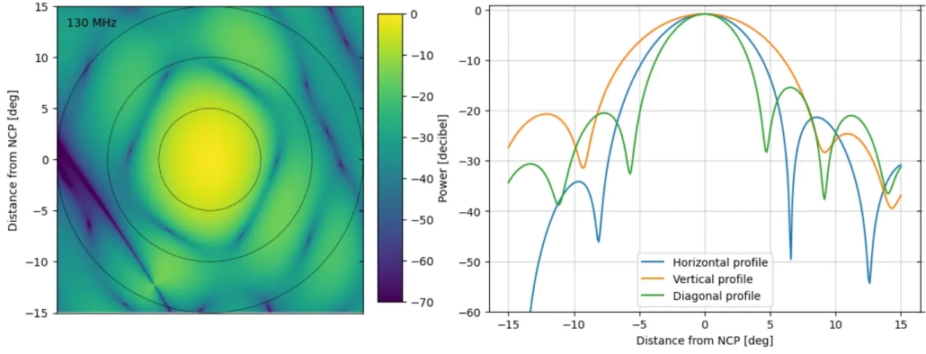
The central 30 degrees of the LOFAR station beam shown earlier is zoomed in here. A LOFAR station beam changes with time, frequency, and direction. This figure shows the beam plotted at a specific time, at 130 MHz, pointed toward the North Celestial Pole (NCP). The left panel displays the 2D beam, while the right panel shows a few of its 1D profiles. All values are given in decibels (dB)—the standard unit for measuring beam power—defined as 20 times the base-10 logarithm of a quantity. The beam value itself is a number between 0 and 1: 1 means maximum sensitivity of the antenna in that direction, and 0 means no sensitivity. In the figure, 0 dB means 1, -20 dB means 100 times less, -30 dB means 1000 times less, and -60 dB means a million times less. From the right panel’s profile, we can clearly see the diameter of the main lobe, which represents the field of view (FoV) of a LOFAR station.

One question from the students at the workshop was: What’s the use of knowing this primary beam? The answer lies in the RIME. In the RIME, the term $\mathbf{B}(l, m)$ is the beam. RIME gives us the complex visibility, but if we want to extract the true sky intensity distribution $\mathbf{E}(l, m)$ from it, we need to apply an inverse Fourier transform (IFT) to $\mathbf{V}(u, v)$. However, this IFT becomes impossible if $\mathbf{B}$ remains inside the integral.

To understand how the beam affects the sky image, assume that our observed image is the product of the true sky image and the primary beam. So, an object exactly at the center of the field will retain its original intensity (since the beam value there is 1), but the farther we move from the center, the closer the beam value gets to zero—and so the object’s apparent intensity decreases accordingly. In a wide-field image, if we want to recover the true values of all objects or pixels, we must divide the entire image by the primary beam. And if we don’t know the beam, how can we divide by it?

In the workshop, we focused only on modeling the LOFAR beam; we didn’t deal with the complexities of removing its effects from an image. That would require much more complicated computations. First, our observations are in the Fourier plane. If, in the real (image) plane, the beam multiplies the image, then in the Fourier plane, the beam convolves with the visibility. To remove the beam’s effect, we cannot simply divide in the Fourier plane—we must perform a deconvolution, which is quite complex. Only after removing the beam’s effect via deconvolution can we apply the IFT to the visibility data and obtain a clean image.

1.4. Timaeus

After a tea break, the eight groups began their projects. The first-day task was to tunnel into CASSA’s HPC server, Timaeus, and—using a Jupyter notebook—plot the Hamaker model of the LOFAR HBA beam. Dutch scientist J. P. Hamaker created this EM-simulated beam model, which, perfect or not, remains the best-known LOFAR beam to date. To plot it, one must first simulate a Measurement Set (MS). In astronomy, real images are stored as .FITS files, and complex visibilities are stored as .MS files. On Timaeus we have already installed synthms for MS simulation and everybeam for plotting the Hamaker beam; the students’ job was simply to use these tools in Timaeus’s Jupyter environment.

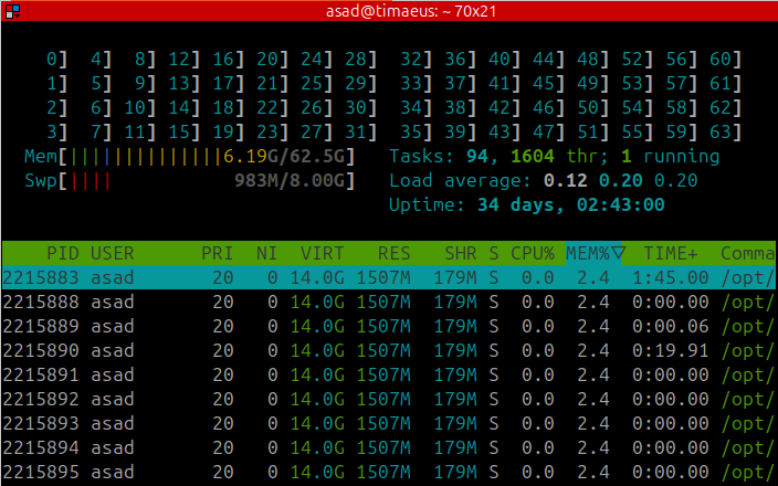
To log into the server, I had set up a common account for everyone. Using SSH, everyone was able to log into that account and navigate to their respective group folders. Along with creating working folders for the eight groups, we also had eight screens open. Each screen was running Jupyter Lab on a unique port. Each group had to tunnel into their respective screen using ssh -N -f -L, and after tunneling, each group was able to open their respective Jupyter notebooks on their laptops. The live server information was visible on the projector screen as shown in the figure above. We had instructed everyone to track the usage of our 64 CPU threads and 64 GB of RAM using this htop output.

Almost all the groups managed to start off well, but disaster struck on our side. Due to some issues in the pre-shared code, MS files were being created for many frequencies, and we hadn’t anticipated that if everyone starts creating beams for each frequency separately, the allocated space on the server would quickly run out. The first day ended with 60 GB of RAM usage, and we know that when 60 GB is exceeded on a 64 GB RAM server, it becomes impossible to do anything properly. So, we ended the first day, dreaming of better server management for the next day.

2. Day Two

On the second day, at 9:30 AM (half an hour late), I shared the actual plan for the group project with everyone. Prior to that, I had stayed up at night solving all the space and memory issues on the server by talking to the TAs. We had created a common beam file for all frequencies as a NumPy array, so no group would create new files. In the morning, I also had to teach everyone a bit about server usage etiquette. The results were great. There were no issues with the server on the second day.

2.1. LoHaZe: LOFAR’s Hamaker-Zernike beam

The day began with a lecture on the project plan: modeling LOFAR’s Hamaker beam using Zernike polynomials. I named this the LoHaZe beam because it is LOFAR’s Hamaker-Zernike beam. A bit of history came into play here. Fritz Zernike started working in the 1920s in Groningen, Netherlands, as an assistant to Jacobus Kapteyn (who was the first to measure the distance from the Sun to the center of the Milky Way). Later, Zernike won the Nobel Prize in Physics for inventing the phase-contrast microscope. It was to model the aberrations of this microscope that he developed the Zernike polynomials.

I did my PhD on LOFAR from 2012 to 2016 at the Kapteyn Astronomical Institute of the University of Groningen. Our science campus was named the Zernike Campus. Later, at the end of 2016, when I moved to Cape Town, South Africa for my postdoc, I used Zernike polynomials to model the primary beam of MeerKAT. During my postdoc, the Python package I developed was used by the students in this workshop, but this time not for MeerKAT, but for modeling the primary beam of LOFAR.

The Zernike polynomials form a sequence where each polynomial unit is orthogonal over the unit disk. Each polynomial in the sequence is identified by radial order $n$ and angular frequency $m$; positive frequencies have a cosine phase, while negative frequencies have a sine phase. The images of the first 10 orders and frequencies of Zernike polynomials are shown above. The general equation can be written in polar coordinates $\rho,\phi$ as:

$$ Z_n^{m}(\rho,\phi) = R_n^{|m|}(\rho) [\delta_{m\ge 0} \cos(m\phi) + \delta_{m\lt 0} \sin(|m|\phi) ] $$

where $\delta_{m\lt 0}$ is a delta function that is 1 for negative frequencies and 0 for all other cases, and $R_n^{|m|}$ is a radial function that depends only on the radius, order, and frequency. Zernike introduced this function to model the aperture of microscopes, and it is also used for aperture modeling in astronomy. As mentioned earlier, the plane of a telescope and the plane of the sky are Fourier transforms of each other, meaning that the aperture plane (the dish mirror or antenna surface) and the primary beam (the sensitivity in various directions) are Fourier transforms of each other. While the beam is the Fourier transform of the aperture, for a LOFAR, it makes sense to model it using the Zernike polynomials instead of the aperture. This is because the aperture of a LOFAR station is not circular but rather rectangular, while the beam is somewhat circular, matching the circular symmetry of the Zernike polynomials.

The students’ task was to decompose the Hamaker beam $B_H(l,m)$, which we created, using Zernike polynomials. After decomposition, they sorted all the Zernike coefficients and selected the best ones to create a beam model $B_Z(l,m)$ using the best coefficients. They did the entire task for the first component ($xx$) of the beam Jones matrix. For decomposition, the Hamaker beams had to be multiplied with the pseudo-inverse of the Zernike polynomials, resulting in the Zernike coefficients:

$$ C = (Z^TZ)^+ Z^T B_H $$

where $^+$ denotes the Moore-Penrose pseudo-inverse and $^T$ denotes the transpose. The number of Zernike modes to be used for decomposition was left to the students. For example, decomposing with 200 modes would yield 200 coefficients. The next task was to select the best 30/40 coefficients. The decision on how and how many coefficients should be selected was also left to the students. After selection, the Hamaker-Zernike beam was reconstructed in the following way:

$$ B_Z = \sum_{i\in L} C_i Z_i $$

where $L$ is the list of selected Zernike modes’ Noll indices ($l$). By using order and frequency, a sequential index for every Zernike polynomial can be created starting from 1, called the Noll index. This makes the calculation much easier; previously, each polynomial required two numbers (order and frequency) for identification, but now only one is needed.

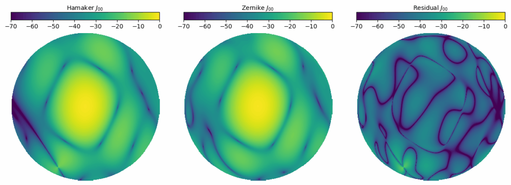
In the first panel of the image above, the original Hamaker beam $B_H$ (up to 15 degrees) is shown. The middle panel displays the reconstructed LoHaZe beam $B_Z$, and the last panel shows the difference between these two as the residual $R = B_H – B_Z$. The power in decibels is given in the color bar. The closer the residual is to zero, the better the LoHaZe model is considered. The residual obtained by selecting the best 40 out of 200 modes has a value of around -30 to -50 decibels almost everywhere, which is quite good.

Here, the students were able to experiment with another aspect. In the image and one-dimensional profile of the LOFAR beam provided in the previous section, a 30-degree area was shown. In such a large angular area, along with the main lobe, two side lobes appear, so higher-order polynomials are needed for modeling. However, to reduce the load of Timaeus, the students limited the beam model to a maximum of 15 degrees. But any group could have done further experiments on this, meaning they could have determined which polynomials would be required for modeling even smaller portions.

The students’ final task was to perform the above decomposition and reconstruction, i.e., the sparse representation for many frequencies between 110 to 170 MHz. Sparse representation was very important for us because, to remove the effect of the beam from visibility, computational efficiency is required. The more efficiently the beam can be described with fewer parameters, the more computationally efficient it becomes. For a 15-degree beam with dimensions of 300 along one axis, there would be a total of 90,000 pixels. However, by using only 40 Zernike coefficients, we are able to recover the values of those 90,000 pixels here.

If we needed to generate beams for 60 frequency channels between 110 and 170 MHz, then the total number of values required would be $90,000 \times 60 = 5.4$ million. However, even if Zernike coefficients need to be stored separately for each frequency, we would only need $40 \times 60 = 2400$ values in total.

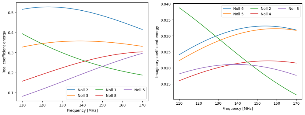
In the figure above, the values of the 5 strongest Zernike coefficients used for modeling the 15-degree Hamaker beam are plotted as functions of frequency. The Noll index for each is given in the legend. The left panel shows the real parts, and the right panel shows the imaginary parts of the coefficients. The variation of the coefficients with frequency is very smooth—something that was not observed in the 30-degree model.

Each group had to compute the residual for each frequency and derive a modeling error. They also had to analyze how this error varied with frequency.

2.2. Group Project

In the CASSA office environment, each group was quite productive. To bring in more of an academic atmosphere, I also clarified the mystery behind the name “Timaeus”—it’s the title of one of Plato’s dialogues. Plato’s collected works were available in the CASSA library. I showed the book and mentioned that anyone interested could read a page or two from Timaeus. I don’t know if anyone actually did, but I did see many flipping through the book.

Realistically, no one had the time to read it. Understanding all the above concepts in one day, completing a full project the next day, and then presenting it—may sound like a lot. But without that kind of intensity, the workshop wouldn’t have felt as immersive, and group members wouldn’t have bonded the way they did. Judging by the photos below, it really seems like they did.

One student mentioned that the best part of the workshop was being able to do a lot of work without any pressure. That’s exactly the kind of environment we try to create—there’s always a lot to do, but everyone contributes as much as they can, and each person takes away something different from the experience. I’m using the word “learning” here in both the positive and the not-so-positive sense.

After the final presentations, I asked everyone to share their main takeaway from the workshop. Hearing their answers made it clear to me that there really is a strong demand for this kind of experience in Dhaka. Before the workshop started, I had said that one or more of the best-performing groups would receive a prize. But after seeing everyone’s presentations, I didn’t feel like singling out any one group. Still, I’d like to incorporate a more rigorous evaluation process in the future.

At the end of the slideshow above, there are photos from all the group presentations. I don’t remember in detail what each group said, but based on the photos, I’ve tried to write something about each of them. Group 1 showed a strong interest in theory—their detailed flowchart suggested a clear inclination toward systematic analysis. Group 2 did a lot of work to determine the right threshold for how many coefficients should be kept. Group 3 thought carefully about why modeling error increases at higher frequencies. Group 4 created a nice plot showing how the error first decreases and then increases with frequency. Group 5 approached the threshold question in a particularly original way. Group 6 put together a well-structured presentation that covered both the theory and the computations. Group 7 explored both thresholding and frequency dependence of the error, and produced the largest number of plots. Group 8 was the smallest group; their results may not have been the strongest, but their thinking was clearly original. So, in the end, I didn’t give a prize to any single group. Honestly, they were all good.

Students came from a total of 15 universities. A few of them had already finished their studies, so they were not officially affiliated with any university at the time, but we still listed their alma mater. A list of all students and TAs can be found here. The largest number of participants came from IUB, which also had the highest number of applications—understandably so, since it’s logistically easiest for IUB students to attend such workshops. The next highest number of students came from the University of Dhaka, followed by the University of Chittagong and the Asian University for Women. In addition, one student each joined from SUST, RUET, MIST, Khulna uni, Ahsanullah, AIUB, BUET, BRAC uni, Daffodil, Edward College, and Hajee Danesh.

Since two Afghan students from the Asian University for Women participated, we had to conduct the entire workshop in English, which turned out to be a great experience for everyone. Although CASSA is based in Bangladesh, it is part of a university—and a university is by definition a place where people from around the world must be able to come together. Over time, CASSA’s international reach will only continue to grow. CASSA is in Bangladesh, but it is not only for Bangladeshis—it belongs to everyone who comes to study, live, or work in this country, regardless of their nationality, ethnicity, religion, gender, or personal identity.

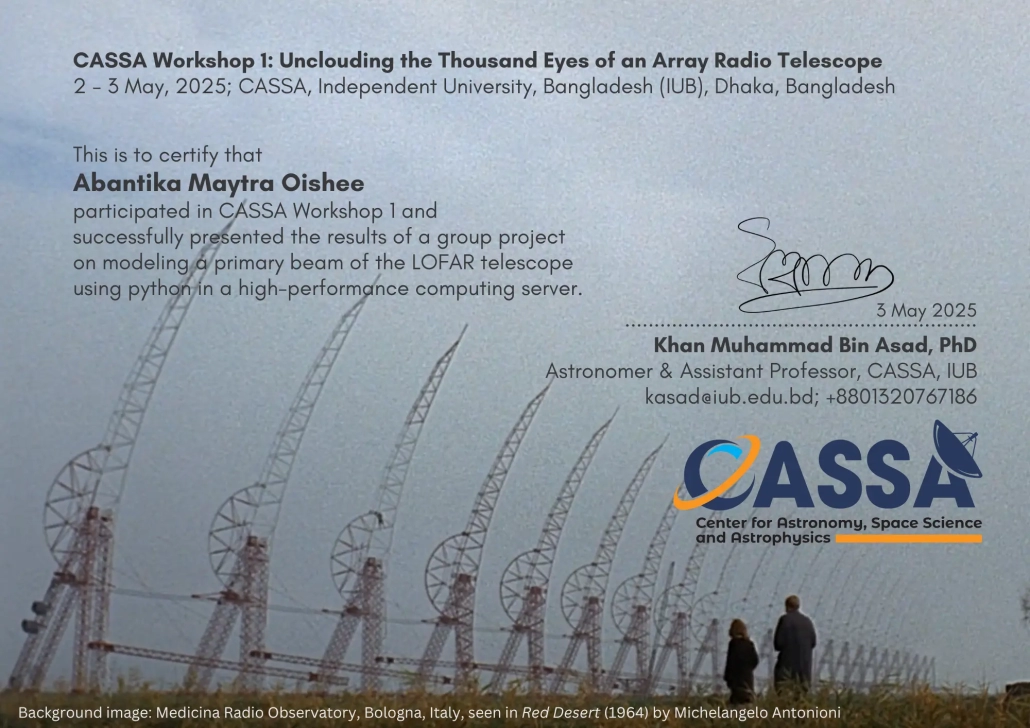
After the workshop, each participant was emailed a certificate. An example is shown above. Like the workshop poster, the certificate’s background features a scene from Michelangelo Antonioni’s 1964 film Red Desert, where the Medicina Radio Observatory near Bologna, Italy, is visible. While radio telescopes have appeared in many films—from James Bond onwards—none use them quite like Antonioni. Red Desert is perhaps the strangest and most striking depiction of human alienation in the modern industrial world. To express this alienation, Antonioni turns to the ART of Bologna. In the scene just after the one shown, the character of Monica Vitti asks a worker, “What are they building here?” The worker replies (paraphrasing here), “they want to listen to the stars with this.” Anyone watching the film will likely feel an existential jolt at that moment.

This is an English translation by ChatGPT from the original Bangla article: কাসা ওয়ার্কশপ ১: মেঘে ঢাকা আর্টের হাজার চোখ

References

Asad et. al., 2021, ‘Primary beam effects of radio astronomy antennas,’ MNRAS, 502, 2970-2983.
Burke et al., 2019, An Introduction to Radio Astronomy, Cambridge UP.
Condon & Ransom, 2016, Essential Radio Astronomy, Princeton UP.
Hamaker, 1996, ‘Understanding radio polarimetry,’ A&A Supplement Series, 117, 137-147.
Smirnov, 2011, ‘Revisiting the radio interferometer measurement equation,’ A&A, 527, A106.
Thompson et al., 2017, Interferometry and Synthesis in Radio Astronomy, Springer Open.
van Haarlem et al., 2013, ‘LOFAR: The LOw-Frequency ARray,’ A&A, 556, A2.