Table of Contents
2. Motion in one and two dimensions
1. Position ($x$)
In order to define the position of a particle at a particular instant in time, we need to first define a coordinate system or reference frame.
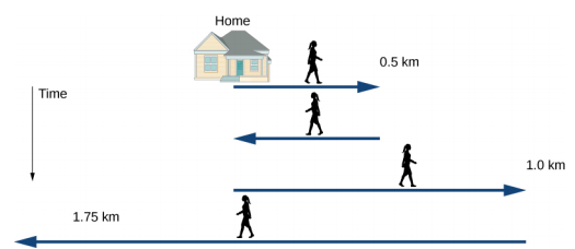
In the above example, home is the origin of a one-dimensional coordinate system and the person is walking from home in different directions in different time intervals as shown below.
| Time $t_i$ (min) | Position $x_i$ (km) | Displacement $\Delta x_i$ (km) |
|---|---|---|
| $t_0$ = 0 | $x_0$ = 0 | $\Delta x_0$ = 0 |
| $t_1$ = 9 | $x_1$ = 0.5 | $\Delta x_1$ = $x_1-x_0$ = 0.5 |
| $t_2$ = 18 | $x_2$= 0 | $\Delta x_2$ = $x_2-x_1$ = -0.5 |
| $t_3$ = 33 | $x_3$ = 1.0 | $\Delta x_3$ = $x_3-x_2$ = 1.0 |
| $t_4$ = 58 | $x_4$ = -0.75 | $\Delta x_4$ = $x_4-x_3$ = -1.75 |
The position is always measured from the origin. It is positive for right-ward movement and negative for left-ward movement. Displacement, on the other hand, is measured with respect to the previous position.
$$ \text{Position } \equiv \text{Current position } - \text{Origin}. $$ $$ \text{Displacement } \equiv \text{Current position } - \text{Previous position}. $$
Displacement is a vector and can be positive or negative, but and the magnitude of the displacement vector is distance.
2. Velocity ($v$)
The position $x$ of a particle at different times $t$ is shown in the following $x-t$ graph.
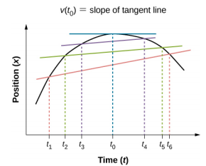
Now the average velocity between, for example, times $t_1$ and $t_6$
$$ v_a = \frac{\Delta x}{\Delta t} = \frac{x_6-x_1}{t_6-t_1} $$
where $x_6$ is the position at time $t_6$ and so on. You immediately see that $v_a$ is actually the slope represented by the red line. Now imagine another average velocity between $t_2$ and $t_5$
$$ v'_a = \frac{x_5-x_2}{t_5-t_2} $$
which is represented by the green line in the graph. In the same fashion, if we keep decreasing the time interval, the slope will keep decreasing and when the interval $\Delta t$ is very close to write the equation for the instantaneous velocity at a particular instant in time $t_0$
$$ v = \lim_{\Delta t\rightarrow 0} \frac{\Delta x}{\Delta t} = \frac{dx}{dt} $$
which is represented by the blue line in the curve. You see that the blue line is a tangent to the curve and it describes the slope at point $t_0$. And this is also the definition the first derivative of the dependent variable $x$ with respect to the independent variable $t$.
$$ \text{First derivative } \equiv \text{ Slope of tangent line}. $$
Velocity is the first derivative of position with respect to time. So velocity is the slope of a tangent line at a particular point on an $x-t$ curve.
Because velocity is the rate of change of position, its unit is meter / second or m/s.
3. Acceleration ($a$)
Now velocity can also change with time and the rate of change of velocity is called acceleration.
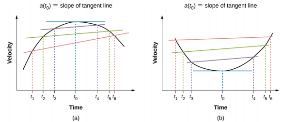
We can perform a similar thought experiment with the above $v-t$ graphs to define average acceleration as
$$ a_a = \frac{\Delta x}{\Delta t} $$
and, similarly, the instantaneous acceleration
$$ a = \lim_{\Delta t\rightarrow 0} \frac{\Delta x}{\Delta t} = \frac{dv}{dt}. $$
So acceleration is sole of a tangent line at any point on a $v-t$ graph. And acceleration can also be expressed as a second derivative of position with respect to time:
$$ a = \frac{d}{dt}(v) = \frac{d}{dt} \frac{dx}{dt} = \frac{d^2x}{dt^2}. $$
Geometrically speaking, the second derivative is related to curvature. So on an $x-t$ graph, the slope of a tangent line at any point gives the velocity, and the curvature at that point gives the acceleration.
$$ \text{Second derivative } \equiv \text{ Curvature}. $$
4. Motion with varying acceleration
Now imagine that the position of a particle is given algebraically by the equation of motion $x(t)=\sin(t)$.
So at time $t=1.57$ s, the position of the particle is $x(t=1.57) = \sin(1.57)=1$ m.
Now we can immediately find the velocity and acceleration of the particle at any past ($t$ negative), present ($t=0$) or future ($t$ positive) time using differential calculus.
$$ v(t) = \frac{dx(t)}{dt} = \frac{d}{dt}(\sin t) = \cos(t). $$
$$ a(t) = \frac{dv(t)}{dt} = \frac{d}{dt}(\cos t) = -\sin(t). $$
The three curves $x(t)$, $v(t)$ and $a(t)$ are represented below by the blue, red and green lines, respectively.
The tangent at time $t=3.14$ s is also shown for each curve using the blue, red and green straight lines. You can see the tangent at other points by hovering your mouse on the graph.
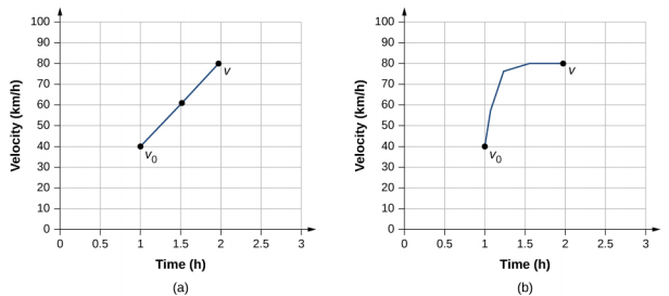
5. Motion with constant acceleration
$$ x = x_0 + v_{av}t. $$
$$ v = v_0 + at. $$
Add $v_0$ on both sides of the above equation to get $v_{av}=v_0+at/2$ and replace this in the first equation.
$$ x = x_0 + v_0t + \frac{1}{2}at^2. $$
Replace $v_av$ and $t$ in the first equation to get
$$ v^2 = v_0^2 + 2a(x-x_0). $$
6. Free falling bodies
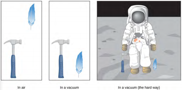
$$ v = v_0 - gt. $$
$$ v^2 = v_0^2 - 2g(y-y_0). $$
$$ y = y_0 + v_0 t - \frac{1}{2} g t^2. $$
7. Integral calculus
$$ x = \int v dt + C_1. $$
$$ v = \int a dt + C_2. $$ Prove $v=v_0+at$ for constant $a$ from this equation.
8. Motion in two dimensions
Position
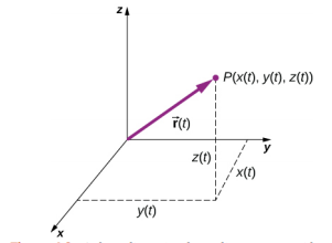
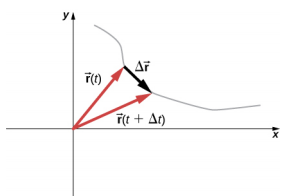
Velocity and acceleration
9. Motion of a projectile
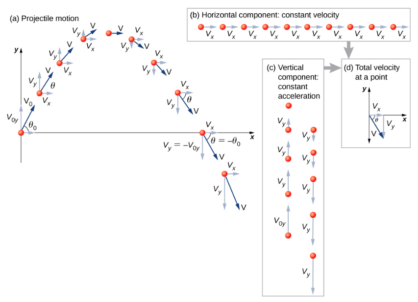
Along the $x$-axis, there is no acceleration and hence $v_{0x}=v_x$ and
$$ x = x_0 + v_xt. $$
Along the $y$-axis, there is constant acceleration, so
$$ y = y_0 + v_{y,av}t = y_0 + \frac{v_{0y}+v_y}{2}t. $$
$$ v_y = v_{0y} - gt. $$
$$ y = y_0 + v_{0y} t - \frac{1}{2} g t^2. $$
$$ v_y^2 = v_{0y}^2 - 2g(y-y_0). $$
Use the 4th equation to get the maximum height
$$ H = \frac{v_{0y}^2}{2g} = \frac{v_0^2 \sin^2\theta}{2g}. $$
Use the 2nd equation to calculate the time of flight
$$ t_f = \frac{2 v_{0y}}{g}. $$
For $x_0=0$ m, $x=v_xt$ and, hence, $t = x/(v_0\cos\theta_0)$. Replace this time in the second equation to get the trajectory
$$ y = (\tan\theta_0)x - \left[\frac{g}{2(v_0\cos\theta_0)^2}\right]x^2 $$
which is an equation of a parabola ($y=ax+bx^2$).
Putting $y=0$ in the trajectory equation gives the range
$$ R = \frac{v_0^2 \sin 2\theta_0}{g}. $$